Testing a fit’s sensitivity to the hyperparameters \(\alpha\) and \(w_{\rm smooth}\)

Context: Interpreting the model’s hyperparameters

The hyperparameters \(\alpha\) and \(w_{\rm smooth}\) affect the fit’s power spectrum estimate (which is itself a prior on the fitted brightness profile). In short, \(\alpha\) acts as a signal-to-noise (SNR) threshold for the maximum baseline out to which frank attempts to fit the visibilities, with a higher value imposing a more strict SNR threshold (thus fitting less of the noisiest data). \(w_{\rm smooth}\) sets the strength of smoothing applied to the power spectrum estimate, with a higher value more strongly smoothing the power spectrum.

Note that the model’s other three hyperparameters, \(R_{\rm max}\), \(N\) and \(p_0\), have a negligible effect on the fit so long as:
- \(R_{\max}\) is larger than the disc’s outer edge (a good choice is \(R_{\rm max} \gtrsim 1.5 \times\) the outer edge).
- \(N\) is large enough to yield a grid of spatial frequency collocation points that extend beyond the longest baseline in the dataset (this also ensures the nominal fit resolution in real space is sufficiently sub-beam). Typical values are \(N = 100 - 300\).
- \(p_0\) is small (\(0 < p_0 \ll 1\); the default is \(10^{-15}\) Jy \(^2\)).

See the frank methods paper for an extended discussion of the model’s hyperparameters.

Performing multiple fits to vary \(\alpha\) and \(w_{\rm smooth}\)

The default value of \(\alpha\) is \(1.05\), and we suggest varying it between \(1.00 - 1.30\). (Though note that choosing \(\alpha = 1.00\) will cause frank to fit a dataset’s entire visibility distribution. For many real datasets, the binned visibilities become noise-dominated at the longest baselines, and fitting these baselines will imprint oscillatory artifacts on the reconstructed brightness profile.)

The default value of \(w_{\rm smooth}\) is \(10^{-4}\), and we suggest varying it between \(10^{-4} - 10^{-1}\).

The fastest way to assess the fit’s sensitivity to \(\alpha\) and \(w_{\rm smooth}\) in practice is to run a fit from the terminal (see the Quickstart), and set alpha and/or wsmooth as a list of values in your .json parameter file. This will produce a figure that overplots the fits for all combinations of your supplied alpha and wsmooth.

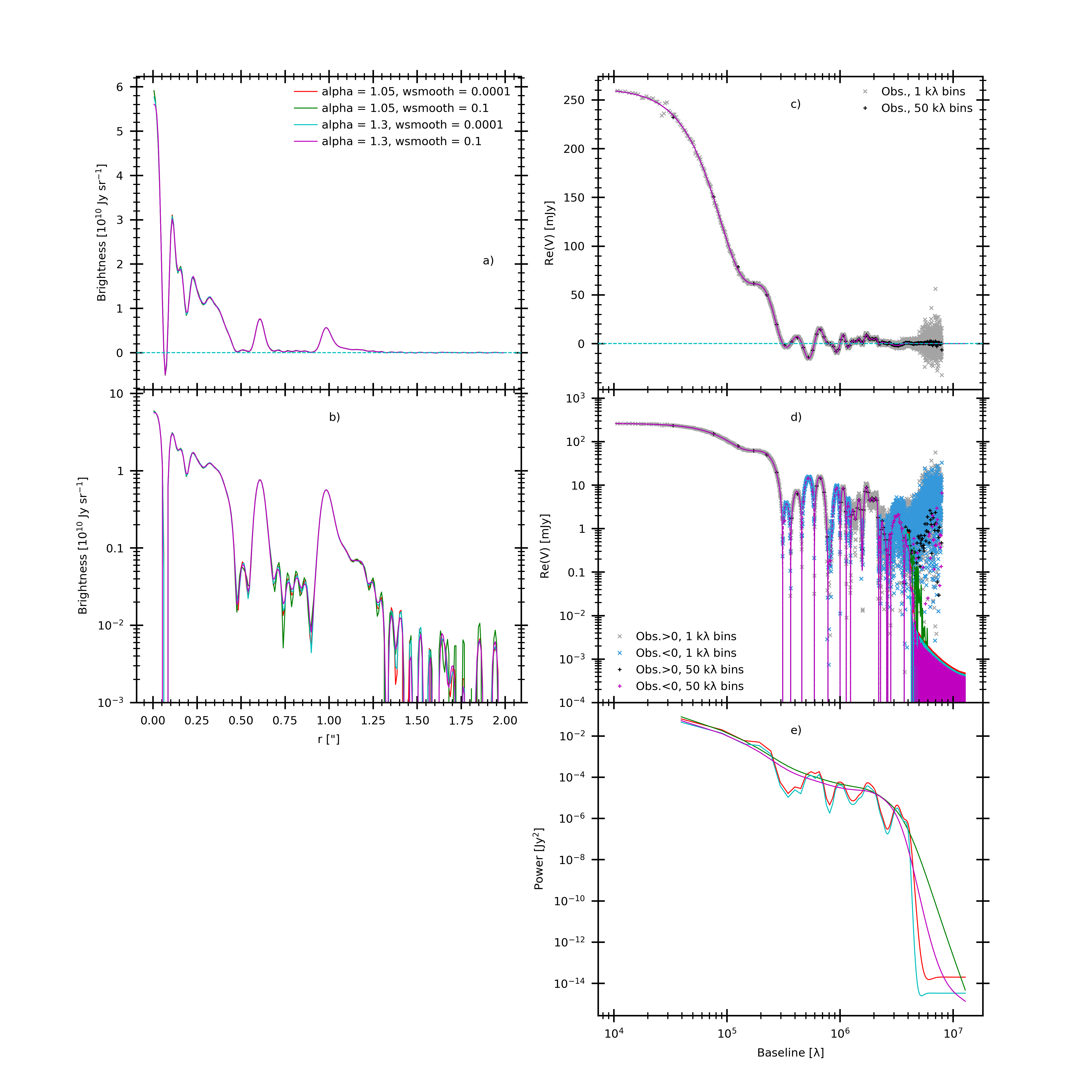
Let’s do this for the DSHARP AS 209 dataset in the Quickstart, using the extrema of the ranges we suggest for \(\alpha\) and \(w_{\rm smooth}\). That is, we’ll set alpha=[1.05, 1.30] and wsmooth=[1e-4, 1e-1] in our parameter file. This will run four fits (for the four combinations of these chosen values), generating this figure,

a) The fitted frank brightness profile for each combination of hyperparameter values. The frank brightness profile for this dataset is evidently only weakly sensitive to our choices for \(\alpha\) and \(w_{\rm smooth}\).
b) As in (a), on a log scale.
c) The visibility domain fits, and the data in 1 and 50 \({\rm k}\lambda\) bins.
d) As in (c), on a log scale, which shows the relatively small variation in how the fits handle the data as they become noise-dominated.
e) The reconstructed power spectrum - which is the prior on the brightness profile - for each fit. Despite the appreciable difference in the power spectrum substructure between the \(\alpha = 1.05\) and \(1.30\) fits, the visibility domain fits in (d) and brightness profiles in (a) are quite similar, demonstrating the effect of the power spectrum as a prior is weak in this case.

Always check a fit’s sensitivity to \(\alpha\) and \(w_{\rm smooth}\)

While these sensitivities can be weak as shown above, a fit’s sensitivity to \(\alpha\) and \(w_{\rm smooth}\) can be nontrivial for lower resolution or particularly noisy datasets. In these cases, the location and amplitude of substructure in the brightness profile can vary with \(\alpha\) and \(w_{\rm smooth}\), so it’s always worth checking how the fit changes over the ranges alpha=[1.05, 1.30] and wsmooth=[1e-4, 1e-1].