Performing a fit

You can interface with Frankenstein (frank) to perform a fit in 2 ways: (1) run the code directly from the terminal or (2) use the code as a Python module.

Perform a fit from the terminal

To perform a quick fit from the terminal, only a UVTable with the data to be fit and a .json parameter file (see below) are needed. A UVTable can be extracted with CASA as demonstrated in this tutorial. The column format is assumed to be u [lambda]     v [lambda]      Re(V) [Jy]     Im(V) [Jy]     Weight [Jy^-2] if the UVTable is in ASCII format (.txt or .dat), or u [lambda]     v [lambda]      V (Re + Im * 1j) [Jy]     Weight [Jy^-2] if the UVTable is in binary format (.npz).

You can quickly run a fit with the default parameter file, default_parameters.json (see below), by just passing in the filename of the UVTable to be fit with the -uv option. The UVTable can be a .npz, .txt or .dat.

python -m frank.fit -uv <uvtable_filename.npz>

If you want to change the default parameters, provide a custom parameter file with

python -m frank.fit [-uv uvtable_filename.npz] -p <parameter_filename.json>

The default parameter file is default_parameters.json. You can get it here, and it looks like this,

{
  "input_output" : {
    "uvtable_filename" : "",
    "save_dir"         : "",
    "save_solution"    : true,
    "save_profile_fit" : true,
    "save_vis_fit"     : true,
    "save_uvtables"    : true,
    "save_figures"     : true,
    "iteration_diag"   : false,
    "format"           : null
  },

  "modify_data" : {
    "baseline_range"   : null,
    "correct_weights"  : false,
    "use_median_weight": false,
    "norm_wle"         : null
  },

  "geometry" : {
    "type"             : "gaussian",
    "fit_phase_offset" : true,
    "fit_inc_pa"       : true,
    "initial_guess"    : false,
    "inc"              : 0.0,
    "pa"               : 0.0,
    "dra"              : 0.0,
    "ddec"             : 0.0,
    "rescale_flux"     : true,
    "scale_height"     : null
  },

  "hyperparameters" : {
    "n"                : 300,
    "rout"             : 2.0,
    "alpha"            : 1.05,
    "p0"               : null,
    "wsmooth"          : 1e-4,
    "iter_tol"         : 1e-3,
    "max_iter"         : 2000,
    "converge_failure" : "warn",
    "nonnegative"      : true,
    "method"           : "Normal",
    "I_scale"          : 1e5
  },

  "plotting" : {
    "quick_plot"       : true,
    "full_plot"        : true,
    "diag_plot"        : false,
    "deprojec_plot"    : false,
    "distance"         : null,
    "force_style"      : true,
    "bin_widths"       : [20e3, 100e3],
    "stretch"          : "power",
    "gamma"            : 1.0,
    "asinh_a"          : 0.02,
    "iter_plot_range"  : null,
    "plot_in_logx"     : false,
    "norm_residuals"   : false
  },

  "analysis" : {
    "compare_profile"  : null,
    "clean_beam"       : {"bmaj"    : null,
                          "bmin"    : null,
                          "beam_pa" : null
                         },
    "bootstrap_ntrials": null
  }
}

Note that anytime you run a fit without specifying -p, frank’s internal default_parameters.json will be used.

You can get a description for each parameter with

python -c 'import frank.fit; frank.fit.helper()'

which returns the contents of parameter_descriptions.json:

{
  "input_output" : {
    "uvtable_filename" : "UVTable with data to be fit. An ASCII file should have columns of: u [\\lambda], v [\\lambda], Re(V) [Jy], Im(V) [Jy], weights [Jy^-2]. An npz file should have columns of: u [\\lambda], v [\\lambda], V [Jy; complex: real + imag * 1j], weights [Jy^-2])",
    "save_dir"         : "Directory in which output datafiles and figures are saved",
    "save_solution"    : "Whether to save `sol` object (see frank.radial_fitters.FrankFitter)",
    "save_profile_fit" : "Whether to save fitted brightness profile",
    "save_vis_fit"     : "Whether to save fitted visibility distribution",
    "save_uvtables"    : "Whether to save fitted and residual UV tables (these are reprojected)",
    "save_figures"     : "Whether to save generated figures selected in 'plotting'",
    "iteration_diag"   : "Whether to return and save diagnostics of the fit iteration (needed for diag_plot)",
    "format"           : "Output file format. Default is the same as for 'uvtable_filename', else choose from 'npz' or 'txt'"
  },

  "modify_data" : {
    "baseline_range"   : "(Deprojected) baseline range outside of which visibilities are truncated, unit=[\\lambda]",
    "correct_weights"  : "Whether to estimate the data's weights (as they may be unknown for mock data)",
    "use_median_weight": "Whether to estimate all weights as the median binned visibility variance (or instead estimate weights using the baseline-dependent variance)",
    "norm_wle"         : "Wavelength (unit=[m]) by which to normalize the (u, v) points (i.e., convert from [m] to [rad]). Not needed if the (u, v) points are already in units of [\\lambda]"
  },

  "geometry" : {
    "type"             : "How the geometry is determined: 'known' if user-supplied, 'gaussian' to fit it with a gaussian, 'nonparametric' to fit it nonparametrically",
    "fit_phase_offset" : "Whether to fit for the phase center",
    "fit_inc_pa"       : "Whether to fit for the inclination and position angle",
    "initial_guess"    : "Whether to use the below values of `inc`, `pa`, `dra`, and `ddec` as an initial guess for the geometry (if `fit_phase_offset` is True or `fit_inc_pa` is True, the respective values below will be used. Guess is only used if `type` is 'gaussian' or 'nonparametric')",
    "inc"              : "Inclination, unit=[deg]",
    "pa"               : "Position angle, defined east of north, unit=[deg]",
    "dra"              : "Delta (offset from 0) right ascension, defined positive for offsets toward east, unit=[arcsec]",
    "ddec"             : "Delta declination, unit=[arcsec]",
    "rescale_flux"     : "Whether to rescale the total flux to account for the source's inclination (see frank.geometry.rescale_total_flux)",
    "scale_height"     : "Parameter values for calcuating the vertical thickness of the disk in terms of its (assumed Gaussian) scale-height: 'h0', 'a', 'r0', 'b' in H(r) = h0 * r**a * np.exp(-(r/r0)**b). 'r0' should be in [arcsec]. Example (replace single- with double-quotes): {'h0': -1.0, 'a': 1.0, 'r0': 1.0, 'b': 1.0}",
  },

  "hyperparameters" : {
    "n"                : "Number of collocation points used in the fit (suggested range 100 - 300)",
    "rout"             : "Maximum disc radius in the fit (best to overestimate size of source), unit=[arcsec]",
    "alpha"            : "Order parameter for the power spectrum's inverse Gamma prior (suggested range 1.00 - 1.50). If a list, multiple fits will be performed and overplotted.",
    "p0"               : "Scale parameter for the power spectrum's inverse Gamma prior (suggested >0, <<1). If 'null', the code will internally choose a sensible value.",
    "wsmooth"          : "Strength of smoothing applied to the power spectrum (suggested range 10^-4 - 10^-1). If a list, multiple fits will be performed and overplotted.",
    "iter_tol"         : "Tolerance for fit iteration stopping criterion (suggested <<1)",
    "max_iter"         : "Maximum number of fit iterations",
    "converge_failure" : "How to treat the case when the fit does not reach convergence by 'max_iter': one of ['raise', 'warn', 'ignore'] to respectively raise an error, raise a warning, or ignore.",    
    "nonnegative"      : "Whether the best-fit nonnegative brightness profile is included in the frank fit solution object",
    "method"           : "The fit method: 'Normal' to fit in linear brighness, 'LogNormal' to fit in logarithmic brightness",
    "I_scale"          :  "Brightness scale, unit=[Jy/sr]. Only used if 'method' is 'LogNormal' -- the 'LogNormal' model produces I('rout') = 'I_scale'"
  },

  "plotting" : {
    "quick_plot"       : "Whether to make a figure showing the simplest plots of the fit",
    "full_plot"        : "Whether to make a figure more fully showing the fit and its diagnostics",
    "diag_plot"        : "Whether to make a diagnostic figure showing fit convergence metrics",
    "deprojec_plot"    : "Whether to make a figure showing the effect of deprojection on the (u, v) points and visibilities",
    "distance"         : "Distance to source, optionally used for plotting, unit=[pc]",
    "force_style"      : "Whether to use preconfigured matplotlib rcParams in generated figures",
    "bin_widths"       : "Bin widths in which to bin the observed visibilities, list of float or int, unit=[\\lambda]",
    "stretch"          : "Type of stretch to apply to swept profile image colormaps, either 'power' or 'asinh'",
    "gamma"            : "Index of power law normalization to apply to swept profile image colormaps (1.0 = linear scaling)",
    "asinh_a"          : "Scale parameter for an arcsinh normalization to apply to swept profile image colormaps",
    "iter_plot_range"  : "Range of iterations to be plotted in the diagnostic figure, list of int of the form [start, stop]",
    "plot_in_logx"     : "Whether to plot visibility distributions in log(baseline) in 'quick_plot' and 'full_plot'",
    "norm_residuals"   : "Whether to normalize plotted visibility residuals in 'full_plot'"
  },

  "analysis" : {
    "compare_profile"  : "Path of file with comparison profile to be overplotted with frank fit (.txt or .dat). Columns: r [arcsec], I [Jy / sr], optional 3rd column with a single error [Jy / sr] or optional 3rd and 4th columns with lower and upper errors",
    "clean_beam"       : "Dictionary of B_major [arcsec], B_minor [arcsec], position angle [deg] of beam to convolve frank profile",
    "bootstrap_ntrials": "Number of trials (dataset realizations) to perform in a bootstrap analysis"

  }
}

That’s it! frank saves (in save_dir) these fit outputs:
- the logged messages printed during the fit as <uvtable_filename>_frank_fit.log,
- the parameter file used in the fit as <uvtable_filename>_frank_used_pars.json,
- optionally, the fitted brightness profile as <uvtable_filename>_frank_profile_fit.txt,
- optionally, the visibility domain fit as <uvtable_filename>_frank_vis_fit.npz,
- optionally, the sol (solution) object (see FrankFitter) as <uvtable_filename>_frank_sol.obj and the iteration_diagnostics object as <uvtable_filename>_frank_iteration_diagnostics.obj,
- optionally, the UVTables for the reprojected fit and its residuals as <uvtable_filename>_frank_uv_fit.npz and <uvtable_filename>_frank_uv_resid.npz,
- optionally, figures showing the fit and its diagnostics as <uvtable_filename>_*.png.

Here’s the full figure frank produces (if full_plot=True in your parameter file) for a fit to the DSHARP continuum observations of the protoplanetary disc AS 209 (Andrews et al. 2018).

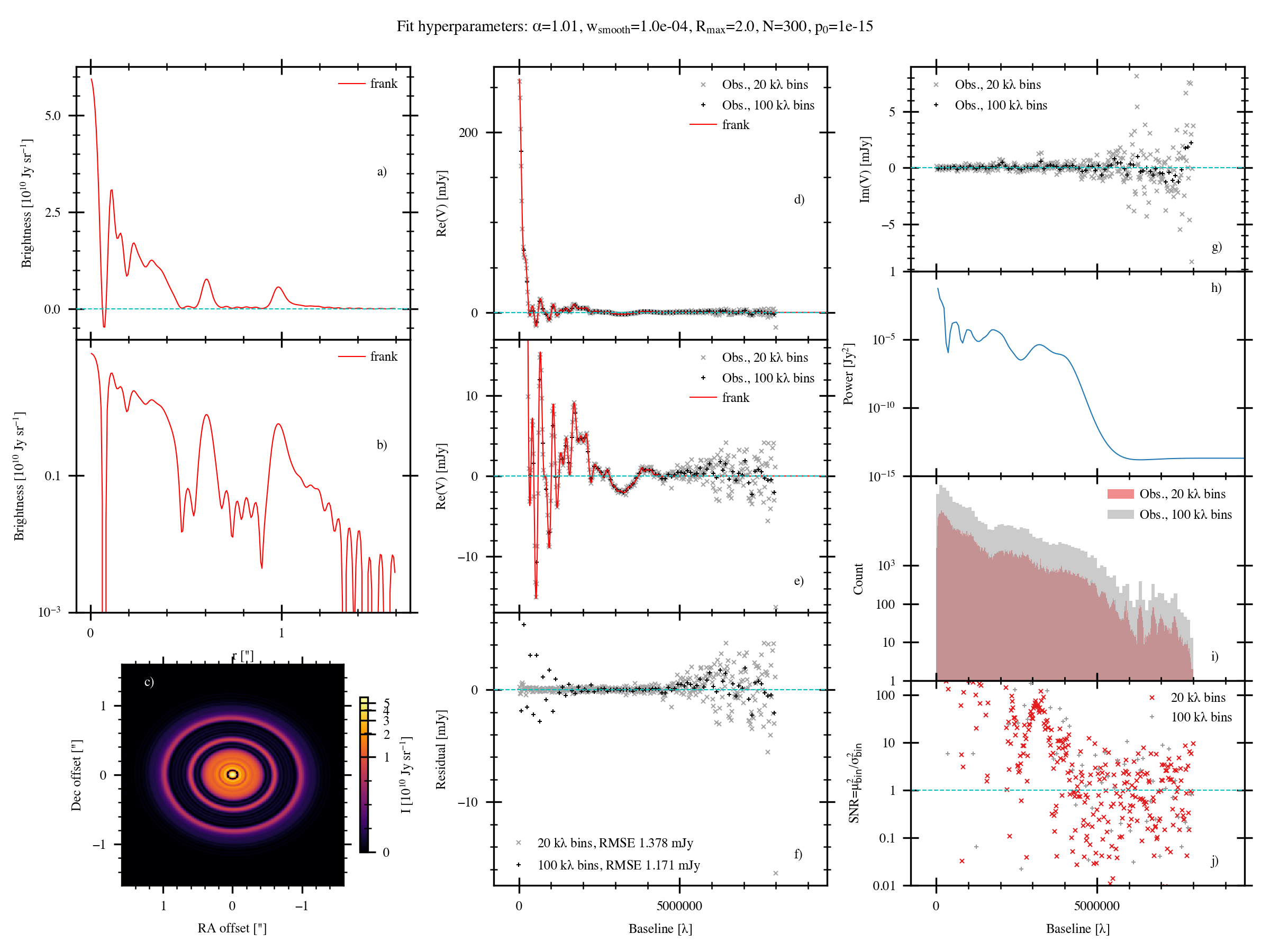
a) The fitted frank brightness profile.
b) As in (a), on a log scale. The oscillations below \(\approx 10^9\ {\rm Jy\ sr}^{-1}\) indicate the fit’s noise floor.
c) The frank profile swept over \(2\pi\) and reprojected. Note this image is not convolved with any beam.
d) The visibility domain fit and the data in 1 and 50 \({\rm k}\lambda\) bins.
e) As in (d), zooming on the low flux region to examine the fit at longer baselines. frank walks off the visibilities as their binned noise begins to grow strongly beyond \(\approx 4\ {\rm M}\lambda\).
f) Residuals between the binned data and the fit. The residuals’ RMSE is given in the legend; note this is being increased by the residuals beyond the baseline at which the fit walks off the data.
g) The (binned) imaginary component of the visibilities. frank only fits the real component, so if Im(V) is large, it could indicate azimuthal asymmetry in the disc that frank will average over.As in (d), on a log scale. h) The fit’s reconstructed power spectrum, the prior on the fitted brightness profile.
i) Histogram of the binned real component of the visibilities. Note how the bin counts drop sharply beyond \(\approx 4.5\ {\rm M}\lambda\), a consequence of sparser sampling at the longest baselines.
j) The data’s binned signal-to-noise (SNR). This begins to dither about SNR=1 beyond \(\approx 4.5\ {\rm M}\lambda\).

Fit for the source geometry

frank fits for the source geometry to deproject the visibilities before fitting for the brightness profile. See here for approaches to the deprojection.

Test the fit’s sensitivity to the hyperparameters

It’s always important to check a fit’s sensitivity to the hyperparameters \(\alpha\) and \(w_{\rm smooth}\). Often the sensitivity is quite weak, but for lower resolution or particularly noisy datasets, the location and amplitude of substructure in the brightness profile can be sensitive to \(\alpha\) and \(w_{\rm smooth}\). You can quickly check this sensitivity by running and overplotting multiple fits in a single call to frank. Just set alpha and/or wsmooth in the parameter file as a list of values. See this tutorial for an example.

Understand the model’s limitations

See this tutorial for an explanation and discussion of the model’s limitations, briefly summarized here:
- Noise in the visibilities can imprint noise on the reconstructed brightness profile (in the above fit to AS 209, this is limited to the regions of flux \(\lesssim 10^9\) Jy sr \(^{-1}\)).
- The fit does not by default prevent regions of negative brightness in the reconstructed profile (as seen above in the AS 209 fit’s innermost gap).
- The model yields a fitted brightness profile whose uncertainty is typically underestimated. For this reason we do not show the uncertainty by default (note its absence in the above AS 209 fit). See here for a fuller discussion and mitigation approaches.

Examine the fit’s convergence

Once a fit has been performed, it can be useful to check its convergence. A convergence test on the inferred power spectrum is performed as the fit iterates, but you can additionally examine convergence of the inferred brightness profile by setting diag_plot=True in your parameter file. frank will then produce a diagnostic figure to assess the fit’s convergence. See this tutorial for an example.

Modify the fit.py script

We’ve run this example using frank/fit.py; if you’d like to modify this file, you can get it here. For an ‘under the hood’ look at what this script does, see this tutorial. If you’d like a video demonstration of the same tutorial (with sound), see here.

Perform a fit using frank as a Python module

To interface with the code more directly, you can use it as a module. The wrapper functions in fit.py do everything we’ll show below, but we’re going to mostly avoid those here, just to show how to directly interface with the code’s internal classes.

First import some basic stuff from frank and load the data (again using the DSHARP observations of AS 209, available as a UVTable - with time-averaging of 30 s and channel-averaging of 1 channel per spectral window - here).

import matplotlib.pyplot as plt
from frank.io import load_uvtable, save_fit
from frank.radial_fitters import FrankFitter
from frank.geometry import FitGeometryGaussian
from frank.make_figs import make_quick_fig

save_prefix = 'AS209_continuum'
uvtable_filename = save_prefix + '.npz'
u, v, vis, weights = load_uvtable(uvtable_filename)

Now run the fit using the FrankFitter class. In this example we’ll fit for the disc’s geometry using the FitGeometryGaussian class. FrankFitter will then deproject the visibilities and fit for the brightness profile. We’ll fit out to 1.6” using 250 collocation points and the code’s default alpha and weights_smooth hyperparameter values.

FF = FrankFitter(Rmax=1.6, N=250, geometry=FitGeometryGaussian(),
                 alpha=1.05, weights_smooth=1e-4)

sol = FF.fit(u, v, vis, weights)

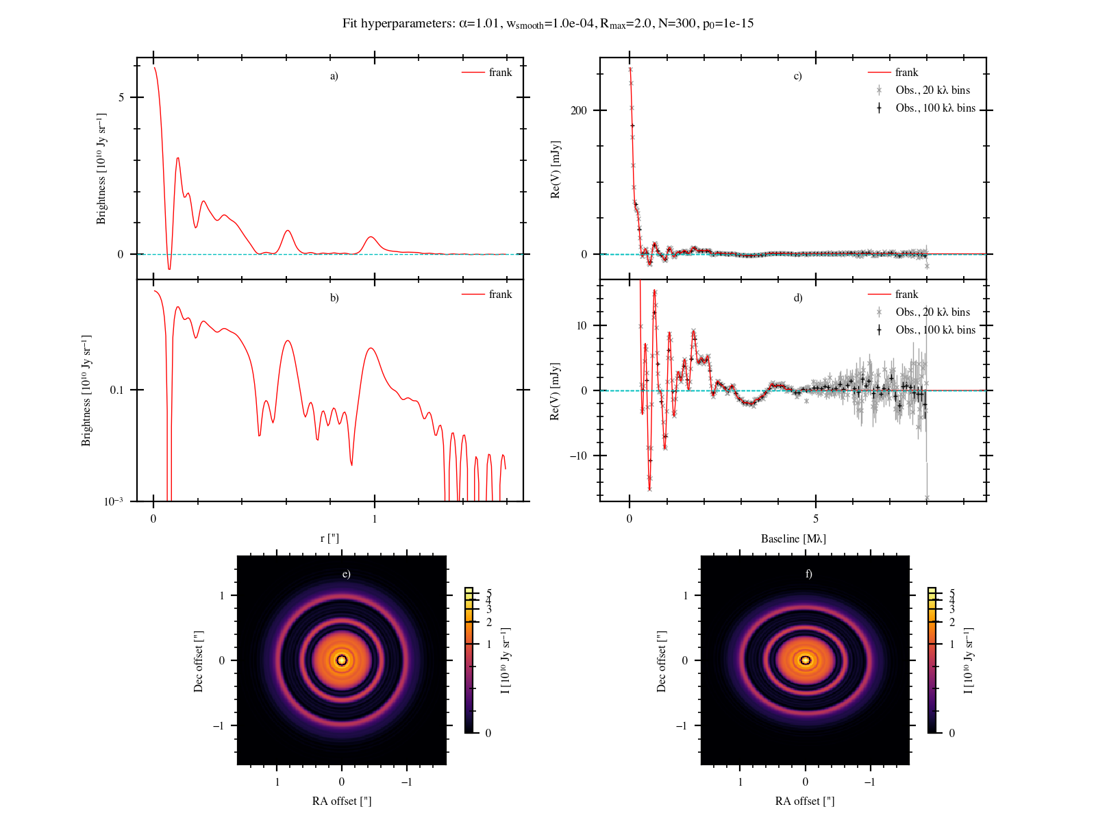
Now make a simplified figure showing the fit (a subset of plots from the full figure above, plus the frank profile swept over \(2\pi\), but face-on, in (e)). When running from the terminal, frank produces this figure if quick_plot=True in your parameter file).

fig, axes = make_quick_fig(u, v, vis, weights, sol, bin_widths=[1e3, 5e4], force_style=True)
plt.savefig(save_prefix + '_frank_fit_quick.png')

which makes this,

Finally we’ll save the fit results.

save_fit(u, v, vis, weights, sol, prefix=save_prefix)